
Why is software tool choice important in RA?
One of the key factors for ensuring a successful resource adequacy assessment is that the software tool choice is appropriate to assess the risks apparent in the region and study at hand. Hence, understanding underlying capabilities of different software tools should allow for identifying the tools best adapted for a given use case. To this end, a request for information (RFI) was put forward by EPRI to better understand key tool functionalities used for resource adequacy analyses today. Numerous tool providers took part in this effort, highlighting the potential for collaboration within the resource adequacy research space. The obtained information, alongside subsequent discussions with both tool providers and other industry stakeholders, is the basis for this overview.

Some of the discussed functionalities, such as the solution methods or the reporting options, are considered core functionalities, as they are relevant for analyses regardless of the use case and resource mix. Other functionalities may only be needed for certain resource mixes or use cases. For example, while complex hydropower modeling may be necessary for hydro-heavy systems, it would not be prioritized for other use cases. The table below highlights a handful of use cases and some of the corresponding tool functionalities that would need to be prioritized in a resource adequacy analysis.
|
If modeling a system… |
Then prioritize… |
|
… with a large amount of energy limited resources |
|
|
… at risk of extreme weather events |
|
|
… in the operational planning timeframe |
|
|
… at risk of shoulder season shortfall events |
|
An objective of this review is to help tool developers and users better understand how their tool’s functionality compares to others in the industry. It should be recognized that tradeoffs are required in most assessment studies because of real-world constraints on resources, data, models, and toolsets. A summary of tool capabilities and options by level of fidelity are provided for all major aspects covered in this overview. The summary is presented as follows:
LEVEL I
Capabilities include the most basic functionalities and representations, which may be sufficient when reliance on a specific technology addressed is low.
LEVEL II
Capabilities are mid-fidelity, which may allow for a realistic representation of certain system characteristics but less so for others.
LEVEL III
The highest fidelity capabilities. This level of tool functionality allows for the most realistic simulations, compared to Levels I and II.
Analysis Approaches
LEVEL I
The solution method employed allows for the evaluation of probabilistic adequacy risk but has key limitations when it comes to the representation of interregional flows and/or the representation of the intertemporal nature of energy limited resources.
LEVEL II
The solution method allows for a fully chronological evaluation of probabilistic adequacy risk and can evaluate multi-area adequacy.
LEVEL III
The solution method allows for a fully chronological evaluation of probabilistic adequacy risk, while also allowing for temporal unit operational limitations such as minimum up/down time and ramping constraints to be considered. Numerous runtime improvements have been implemented to ensure computational tractability.
This includes many dispatch-based fully chronological Monte Carlo methods.
Convolution Methods
Convolution is an analytical method that calculates a total available capacity distribution by convolving together the distributions associated with available capacity for each unit in the system. This resulting distribution is calculated for every time interval of the resource adequacy analysis, and a loss of load is identified if the available capacity is lower than the demand in the time interval being considered. It considers the full distribution of all discrete system states and is typically characterized by the following properties:
-
Convolution Methods are deemed to be a computationally efficient way to exhaustively enumerate all possible states in a given interval in comparison to other approaches (especially Monte Carlo Methods).
-
The intertemporal nature of power systems operations and the asset-specific performance impacts are ignored since each time interval is assessed independently of all others. This limits the ability to accurately consider energy storage operations.
-
It is generally not well suited to multi-area resource adequacy modeling, as that increases the number of unique system states and thus the computational complexity of the problem.
Monte Carlo Methods
Monte Carlo methods rely on repeated random sampling to calculate adequacy risk indices. Here they refer to a general class of models where in each replication (or sample), uncertainty variables such as forced outage occurrences are assigned a random value from user-specified probability distributions. This process is applied repeatedly while assigning different values each time to the variables in question, until an acceptable level of statistical precision is achieved. Adequacy risk metrics are then calculated as the average of the accumulated replication data.
Although the final solution is an approximate one (in contrast to the convolution method which considers all possible system states), this method allows for simulating of more complex problems than would be possible analytically, including those with inter-regional and intertemporal constraints. Note that the more replications across the distribution are performed, the more the approximate nature of the Monte Carlo method is reduced. Certain existing RA tools were initially created as production cost tools that then evolved to include resource adequacy functionality by adding a Monte Carlo component to existing optimization engines, other Monte Carlo tools were developed independently of production cost functionality. Monte Carlo methods can be divided into several approaches, classified as follows:
The non-chronological Monte Carlo sampling methods randomly samples system states for every time interval of a simulation to assess system adequacy, however, this is not conducted in a chronological manner. Therefore, these tools:
- Are the least computationally intensive of the Monte Carlo sampling methods.
- Easily represent inter-regional power transfer limits and line outages.
- Do not account for the chronological nature of system components (e.g., power plant outages states and storage operation).
Compared to other approaches, non-chronological Monte Carlo sampling methods are not a widely used method in the tools surveyed.
The heuristics-based chronological Monte Carlo methods simulates a chronological system evolution, allowing for tracking of outage states and the state of charge of energy-limited resources. Often-used heuristics include an assumption that all thermal units are available when not on outage (not considering unit ramp and minimum up and down constraints), and an assumption that energy storage is fully charged and available for discharge at the start of a loss of load event. Heuristics-based chronological Monte Carlo methods:
- Are more computationally intensive than the convolution or non-chronological Monte Carlo methods.
- Remain much simpler (and therefore less computationally intensive) than a dispatch-based Monte Carlo method.
- Are well adapted to the study of capacity adequacy but may be less well suited to the consideration of energy adequacy and flexibility adequacy, as they do not model a full economic dispatch process, which may require economics to understand how the system is likely to be positioned during periods of high risk.
Chronological dispatch-based Monte Carlo methods are a commonly available method in RA tools. All the tools in this category dispatch the system based on system costs and can model several inter-temporal unit constraints such as unit ramp rates and start times. A high penalty cost is associated with unserved energy, effectively ensuring that load loss events are minimized. Most tools in this category minimize total system costs using an optimization algorithm. Due to these facts, these approaches:
- Are computationally intensive compared to other methods.
- Provide a more accurate depiction of power systems operations than other approaches.
- Can consider economic dispatch.
If a user wants to dispatch the system to minimize unserved energy only, they can do so by setting all other system costs to zero. Note that the user is often the one responsible for assigning this penalty cost, and as such must be thoughtful of how it interacts with other penalty costs (for example, penalty costs for transmission line rating violations, or for ancillary service shortfalls, when modeled).
It is important to keep in mind that tools using Monte Carlo dispatch-based method are not automatically more accurate than tools employing other solution methods. Ultimately, accuracy depends modeling assumptions, e.g., simplifications to decrease computational burden, but also on the representation of other key resource adequacy features, such as thermal unit outage and weather uncertainty representations. However, for certain types of studies, particularly those where energy adequacy is important, Chronological Monte Carlo Sampling Dispatch-Based provide inherent advantages.
Note that not all dispatch-based Monte Carlo methods are automatically categorized as Level III tools – users have to be able to run a sufficiently large number of probabilistic replications to achieve convergence in a time-effective manner for an analysis approach to qualify as Level III.
Alternative Approaches
While certain tools identify as pure either Convolution or Monte Carlo techniques, several solution methods that were reported in the request for information do not unambiguously identify as one these two approaches.
Avoiding the complexity of a full chronological Monte Carlo simulation, one of the surveyed tools approximates it in a multi-step approach. First, the resource adequacy assessment is performed in a non-chronological Monte Carlo manner. In this assessment, each replication is evaluated for each time block with available capacity being subject to failure probabilities. A pseudo-chronological analysis can subsequently be executed to investigate the duration and frequency of outages. For this purpose, outages identified in the preceding non-chronological step are analyzed in more detail by back-tracking hour by hour the start and end times of loss-of-load events considering failure and repair rates of each component. In systems where small storage devices can contribute to resolving shortages, operation of these devices can be optimized for the duration of the failure state identified in the preceding pseudo-chronological step, allowing for some of the advantages of Monte Carlo simulations, but reducing runtime. Note that unit commitment chronology is not represented in this approach.
One of the surveyed tools uses a simplified solution method to reduce computational complexity. Again, in this method, storage and demand response are considered chronologically, but not unit ramp rates or minimum up/down times. For this solution method, the tightest system hours are identified based on estimated average plant availability (excluding unplanned outages) for each weather pattern. The user can either choose to select a certain number of system hours for consideration or can select to consider all hours below a certain reserve margin percentage. The solution method then selects both the tight system hours identified as well as their adjacent hours for further analysis, with the number of adjacent hours a user-set parameter which should be set based on the maximum short-duration unit length in the system being modeled. This approach allows for the number of considered timesteps, and therefore the computational complexity, to be reduced. In the following step, plant outages are randomly sampled and aggregated into blocks of available capacities and associated probabilities for each study region. Outage rates are used for specific plants, whereas average availabilities are assumed for aggregate plants. This method resembles to an extent Monte-Carlo simulations, however, the user-defined number of capacity blocks is typically smaller than the number of generators in a system. To account for regional effects, available capacity blocks for each region are randomly sampled and the joint relative probability of the system is calculated by multiplying the probabilities of each of these blocks. Short-term storage operation and transmission flows are then optimized over the identified critical periods and their adjacent hours to minimize unserved energy.
Even though standard Convolution Methods are generally not well suited to multi-area resource adequacy modeling, the “Convolution Method Using Monte Carlo-Derived Inputs” allows for multi-area modeling by calculating each area separately using a classic convolution method, and then considering inter-area exchanges in post-processing. It uses a convolution model to evaluate the adequacy of a system but uses a Monte Carlo sampling analysis to calculate unit-level availability distribution profiles for each hour of the analysis. Thermal resource availabilities are sampled on an hourly basis using two-state Markov modeling methodology (which incorporates both time to failure and time to repair), and the results of this sampling are used to create a different unit availability distribution profile for every hour of the analysis. Historical hourly data is used to create hourly historical probability distributions for all area-level demand profiles and variable renewable energy profiles. Once area-level adequacy is calculated, the solution method considers inter-area balancing by allowing for transfers from neighboring areas and their immediate neighbors if excess generation is available and transfer capability is sufficient.
Most respondents to the RFI use dispatch-based chronological Monte Carlo methods in their software tools, as shown below.
As energy and flexibility adequacy become more important, the industry is moving towards the use of dispatch-based chronological Monte Carlo methods. It can also be noted that this is partly since several of the tools surveyed were initially developed for production cost analysis, and later developed resource adequacy functionality, such that the Monte Carlo based method was a natural step. One of the tools surveyed as part of this work used a heuristics-based Monte Carlo method upon first discussions but has since transitioned to a dispatch-based Monte Carlo method. Note that multiple options in the figure above were selected for tools with multiple solving modules available to the user.
Ensuring Computational Tractability
Probabilistic runs are computationally very expensive, especially as resource models are getting more complex and there is an increasing push to consider energy and even flexibility adequacy within the probabilistic resource adequacy framework. To this end, many of the surveyed tools have implemented methods to facilitate computational tractability. These include options for parallelization or multi-threading, various methodologies to screen for at-risk adequacy hours, methods to easily simplify or tune the model for probabilistic analysis, and the use of high-performance or cloud-computing.
Many of the surveyed tools allow for parallel processing of resource adequacy runs. This can allow for multiple weather years or even individual replications to be run in parallel. Some of the tools surveyed allowed for split runs, i.e., the ability to portion replication-level runs into smaller, independent subproblems. For example, a problem of 8760 hourly timesteps could be sectioned into 52 weekly subproblems of 168h (or e.g., 192h to account for a period of look ahead horizon). Note that while this practice is commonly used, this methodology alone is not suitable to represent chronology over longer timeframes relevant to represent the operation of generators with longer time constants, e.g., hydroelectric units or seasonal energy storages. Care should be taken to consider how tools using this practice approach this challenge, with information on the topic found in the Hydropower section of this document. Modeling choices for energy storage are also discussed in the modeling guidelines document, to describe accuracy of different models.1
Several of the tools evaluated have developed methodologies to screen for at-risk adequacy hours. This can range from simplistic methodologies, such as foregoing runs of lower load uncertainty levels if higher load uncertainty levels did not yield shortages in an hour, to more sophisticated methodologies, such as applying variance reduction techniques using purpose designed stratified sampling. One common approach consists of screening for periods at risk using a simplified representation of the system, and then performing more detailed analyses of these periods. This can be accomplished by incorporating a simplified representation of thermal resource unavailability in the initial system runs, or by ignoring certain operational constraints initially. As with the split run capability discussed above, care should be taken to ensure long-duration energy-constraints such as seasonal hydro and energy storage are appropriately captured.
Probabilistic analysis tools are increasingly being called upon to incorporate more complex resource models. As such, the ability to easily simplify and tune the model for probabilistic analysis, especially in tools initially created for production cost simulation applications, is key. This requires some level of technical know-how on the user’s part to sufficiently tune optimization parameters and to understand which level of modeling detail is important to include for a specific study. The Technology and System Component Model Selection Guidelines site can help guide these decisions. Additionally, certain optimization setups, such as the use of solver warm starts (e.g., providing an initial point for the subsequent rolling horizon window) and the use of linear or dynamic programming solution methods instead of MIP programming can improve computational runtime. Finally, a useful capability for these tools is the ability to easily switch from a full optimization model to a “must-run” or “commit all” model, in which a full economic dispatch is not considered, for initial setup or testing purposes.
Several tools evaluated as part of this initiative have processes in place to allow the user to leverage high power computational resources such as high-performance clusters or cloud-computing. This capability to execute model runs remotely offers more flexibility to outsource computational time and leverage high performance computing. However, firewalls, data security and IT restrictions can be a hurdle.
Read more:
Risk Metric Reporting
LEVEL I
The tool outputs standard risk metrics like LOLE, LOLH, and EUE for both the full system and for each region modeled.
LEVEL II
The tool outputs standard risk metrics like LOLE, LOLH, and EUE for both the full system and for each region modeled. Additionally, it can output replication-level results to allow the user to calculate custom metrics.
LEVEL III
The tool automatically outputs both standard risk metrics and custom advanced risk metrics defined by the user (for example: LOLE95) for both the full system and for each region modeled. In addition to outputting replication-level results, tools in this category can output results at various levels of granularity (temporal, by weather year, etc.).
Historically, loss-of-load expectation (LOLE) was the only metric reported across many systems. However, there is an increasing body of research that demonstrates that using a suite of resource adequacy metrics is essential to ensuring a full understanding of system risk. Most of the surveyed tools include standard risk metrics outputs. Several tools also have the capability to automatically output several less commonly used risk metrics. The table below provides an overview of the commonly and not commonly output risk metrics. For further information on the various metrics, please refer to the Metrics page.
Commonly reported risk metrics | Not commonly reported risk metrics |
|
|
Note that these metrics may be output with varying levels of ease from one tool to another: the intent of the survey question was to evaluate which metrics are automatically output by tools as part of their standard output, but certain survey respondents included metrics that are available through their tool but may require some level of customization or calculation on the user’s end to output. Users are encouraged to discuss with tool providers about the metrics available and how they can be calculated.
Read more:
Reported Granularity
Another variation from one tool to another is the granularity at which each of these metrics can be output. This refers to the temporal granularity (e.g., annual up to daily granularity), the results on each replication level, by geographical area, or by weather year (useful when evaluating the impact of potential extreme weather events on system risk).
Not every tool has all outputs available, but users are encouraged to understand and use what is available to them to gain more insight into the nature of the outages they observe. The table below illustrates the possible temporal and replication-level granularity reporting options available in resource adequacy tools.

Temporal Granularity
Regarding the temporal granularity, several tools allow for key metrics to be output at both an annual and monthly granularity, while a few tools additionally allow for daily and weekly granularity. Several of the tools surveyed allow for metrics to be output as averages by hour of day. Many tools allow for results to be output by hourly granularity, thus allowing for the user to calculate a number of custom metrics and visualizations in post-processing. Clearly, allowing for more granular outputs can enable more insightful analysis into the types of shortfalls, but there may be data limits or other computational challenges in outputting such detail.
Application-Level Results
Although many tools do not automatically output by replication due to the large amount of data this represents, many allow replication-level results to be pulled by the user if desired. These replication-level results are more or less straightforward to extract depending on the individual tool interface. Additionally, several tools also allow the option for replication-level results to be output as an annual average by replication, or an hourly average across all replications. This reduces the amount of data output to the user, while also providing relatively detailed results for review.
The ability to output replication-level results is useful not only for debugging purposes, but also if calculating custom risk metrics beyond the ones automatically output by the tool. Post-processing scripts can either be appended as part of a custom add-on to the tool, or calculated separately, after all replication-level results have been retrieved. EPRI has developed an online tool which can be used in post-processing to visualize several resource adequacy metrics based off hourly replication-level results.1 Alternatively, a handful of the tools surveyed allowed the user to easily define custom advanced risk metrics within the tool interface itself.
Other Risk Metric Reporting
One of the tools evaluated as part of this initiative allows for resource adequacy metrics to be output on a nodal level, allowing for the marginal effect of nodal load variations on unserved energy to be captured. Similarly, although less common, the ability to automatically output key risk metrics by weather year is useful when evaluating the impact of potential extreme weather events on system risk.
Read more:
1 EPRI, "Resource Adequacy Viewer Tool (RAVT) v1.0 (3002026144)," Palo Alto, CA, 2023.
Generator Forced Outage Modeling
LEVEL I
Only allows for fixed or seasonal generator outages to be defined. Allows for either no or only limited modeling of partial generator outages.
Uses either an outage rate probability methodology, or a Markov-based chronological outage modeling methodology or similar (exponential, Weibull, or non-parametric distribution). Does not allow for start-up failure or coincident outages to be modeled.
LEVEL II
Allows for the modeling of either full or partial generator outages that can be varied for every timestep of the analysis, which allows for correlated weather impacts to be represented in thermal generators. Uses a Markov-based chronological outage modeling methodology or similar (exponential, Weibull, or non-parametric distribution). Allows for start-up failure and coincident outages to be modeled.
LEVEL III
Allows for the modeling of either full or partial generator outages which can either be varied for every timestep of the analysis or can be directly linked to key variables such as temperature. Uses a multi-state Markov transition matrix forced outage modeling methodology. Allows for condition-based start-up failure and coincident outages to be modeled.
All respondents to the RFI have tools that can model and evaluate the impact of forced generator outages on system adequacy risk. The methods for modeling these forced outages do vary from one tool to another, however, and in some cases, a tool may offer several forced outage modeling methodologies depending on the ultimate study goal. Many of the generator forced outage modeling capabilities surveyed are either Level I or Level II. Part of the reason for this is that many of the survey respondents develop tools which are used for both resource adequacy and production cost analysis. Accurate outage modeling representation, while long considered a core functionality of resource adequacy analysis, is less important for many production cost analyses. Accurate outage modeling was identified as a key resource adequacy tool gap by many of the respondents.
Unit Unavailability
Unit unavailability can be due to several factors, including forced outages (defined as a state a unit enters when it is no longer capable of delivering energy to the grid), partial outages (defined as an unscheduled forced reduction in unit capacity), and startup failures (defined as a forced outage due to a failure that occurred during a unit’s startup procedure). Depending on the tool, unscheduled generator unavailability occurrences are either calculated in pre-processing, or dynamically for every time step of simulation. A unit unavailability schedule calculated in pre-processing means the tool has perfect foresight of all future outages and can adjust system unit commitment and dispatch accordingly. For example, it may start-up or ramp up a unit in anticipation of a future forced outage event, which isn’t aligned with real-world operations, where this would not be known. This may result in an overoptimistic result as compared to an algorithm without perfect foresight; accounting for unscheduled unit unavailability only as it happens is more realistic. Alternatively, in some tools, unscheduled generator unavailability is identified at the start of the user-defined optimization window, giving the solver perfect foresight within the optimization window but not outside of it.
The figure below illustrates the primary outage modeling tool capabilities practitioners should be considering when modeling extreme weather events. These include both a robust core outage modeling functionality as well as sufficient add-on functionalities as to accurately represent system behavior during extreme events. Note that not all analyses will require every single functionality detailed in this figure. For example, coincident outage modeling may not be necessary in systems not prone to natural gas pipeline shortages. The accuracy of the available core outage modeling functionalities is represented graphically, with methodologies ranked from least accurate to most accurate. The Markov-based modeling methodology is the most used and appears to accurately represent both the probability of outages and the impact of varying outage repair times. The generalized distributions methodology and the non-parametric distribution methodology are both more comprehensive, as they extend beyond exponential distributions to also allow the user the choice of other probability distributions. Several simplified methodologies were also offered, including the outage probability rate methodology which, while allowing for the probability of outages to be represented, does not accurately represent the repair behavior of the generator on outage. As such this method is best reserved for non-chronological modeling uses only. Several other simplified methodologies, such as the capacity derate methodology and the convergent outage methodology should be reserved for deterministic analyses, or analyses in which a full resource adequacy analysis isn’t required. Indeed, although these methodologies have their utility, they fail to accurately represent all outage possibilities, particularly tail events, which are of high interest to any resource adequacy analysis.

Figure: Outage modeling tool capability considerations for extreme weather modeling
Forced Outage Modeling
Forced outage representation is approached differently depending on whether the solution method considers study hours chronologically or not. Many of the outage modeling methodologies are often used when the resource adequacy solution method considers hours chronologically. These methodologies recognize the fact that a unit’s state in each hour is dependent on its state in the previous hour and influences its state in the future hour. There is some variation across tools as to how these outage modeling methodologies are implemented, but at its core, they consider both how likely a unit is to go on outage as well as how long it takes it to recover from an outage. The measure of how likely a unit is to go on outage can be input as either a mean time to failure (MTTF) or an equivalent forced outage rate - either EFOR which is the probability that a unit will be unavailable due to forced outages, or EFORd which is the probability of unavailability for times when there is demand on the unit to generate. The measure of how long it takes a unit to recover from an outage can be input either as a mean time to repair (MTTR) or an average number of outages over the study period. Alternatively, a state transition matrix can be used which indicates the probability of moving from one availability state to the next. The forced outage modeling methodologies of the tools evaluated are further discussed below.
Many of the tools surveyed use a Markov process to stochastically determine generator forced outages. A special property of the Markov process is that, while each new state depends on the one before it, new states do not depend on any states before the previous one. This special property is referred to as “memorylessness” and is limited to geometric distributions of non-negative integers and the exponential distributions of non-negative real numbers.
Several tools surveyed allow for other distributions in addition to a traditional exponential distribution. Less commonly used probability distributions include the Weibull distribution (a more general distribution than the exponential distribution, where the failure and repair rate is proportional to a power of time, rather than constant as it would be for an exponential distribution) and the uniform distribution which allows outages to vary uniformly around a certain duration.
Two of the tools surveyed instead ask the user to provide a discrete set of possible times to failure and times to repair, often based on historical NERC GADS (or similar) outage data. This discrete set of possible times to failure and times to repair form a histogram, which the tool randomly selects from for each draw. A third tool asks the user to provide a probability of occurrence for a discrete set of outage failure durations.
While the user inputs a forced outage rate and a mean time to repair, similarly to other methods, this methodology adjusts outages in such a way that each replication run has a forced outage rate exactly equal to the EFOR entered by the user. As such, although the outage occurrence is assigned randomly, the amount of time a unit spends on outage for each replication is fixed. This allows for more repeatable results and is sometimes used if a user cannot run enough Monte Carlo replications to achieve sufficient statistical precision. However, this methodology does not capture all possible outage scenarios, as any scenarios with a higher or lower amount of time on outage than the EFOR are not modeled. As such, it fails to capture tail events, which are of high interest to many system planners, and the fact that an EFOR number represents the average of a wide range of outages in any given year.
This outage modeling methodology does not incorporate any chronological consideration of outage probability. The probability of outage (whether full or partial outages) is input without providing information on the duration of the outage.
This methodology is traditionally used with convolution methods, in which every hour is considered independently. However, one of the tools evaluated used this outage methodology in combination with a Monte Carlo method: they run each week of the study period independently, and if a unit is on a forced outage, it is on outage for the full week.
This outage modeling methodology applies the forced outage rate input by the user as a constant capacity derate across all time intervals of the simulation. Although this methodology results in the appropriate amount of capacity derated due to forced outages on average, it does not realistically represent the impact that forced outages have on the system: a unit which is on forced outage for part of the year is harder for the system to prepare for than a unit which is derated by a small amount over the full study period. This is typically more useful for resource planning studies or similar, where an approximation of unit outages may be sufficient.
One tool respondent did not have any forced outage modeling methodology available. Instead, they had the capability for generator capacity to be specified on an hourly basis. As such, a user would need to set up a pre-processing script to create outage patterns for all generators and input them as hourly capacity profiles to be able to analyze the impact of forced outages on resource adequacy. In theory, this could allow for complex forced outage modeling methodologies to be represented, such as allowing for correlated outage modeling and full representation of transition rates from one outage state to another, while in practice this may be very time consuming without a well-developed pre-processing script and suitable data.
Partial Outage Modeling
While all tools surveyed allow for the option to model generator forced outages, many do not allow for the option to directly model partial forced outages, which are outages associated with a reduction in capacity, rather than full unit unavailability (these are sometimes referred to as 'forced capacity derates’ and differentiated from 'capacity derates' above in that they only happen for a specific time rather than the full simulation period). The most accurate way to define partial forced outages in a chronological consideration is using a multi-state Markov transition matrix. This allows for relationships between outage states to be fully defined, something that is not possible in any of the other outage modeling methodologies. This allows for discrete combinations to be enforced, for example that a unit when returning to service always goes to full output and never a partial outage state. Note that a 2-state Markov process, which can be characterized either through a state transition matrix or by a mean-time-to-failure and a mean-time-to-repair value, is a subset of a multi-state Markov process, as illustrated in the figure below. A MTTF/MTTR process allows for the use of a generalized outage distribution, but if it uses an exponential distribution, it is considered a 2-state Markov process.

Figure: Intersection of Markov processes and MTTF/MTTR processes
Several tools considering outages chronologically instead allow the user to define a separate time to failure and time to repair (or similar characteristics) for partial outage states than for a full forced outage state. However, this does not allow for the transitions between outage states to be fully characterized.
When forced partial outage modeling is not available, a workaround is sometimes used to model multiple units within a plant or model a unit as being comprised of multiple sub-units, thus allowing the user to associate a forced outage rate to only a portion of the plant. However, this can result in complicated implementation, depending on the level of detail needed. For example, a coincident outage would need to be specified to model a plant-wide outage under this configuration.
Startup Failure Modeling
Startup failures are an unscheduled outage type where the affected unit is fully unavailable due to a failure that occurred during its startup procedure. The ability to model start-up failure is not a widespread capability amongst resource adequacy tools. Only two of the tools reported having this capability at the time they were surveyed. Note that only one of these allowed for a time to repair value to be defined, the other assumed the generator would be available again in the next commitment cycle.
Start-up failure modeling may become increasingly important in systems with significant ramping requirements, when multiple units start in close succession to meet a net load ramp, potentially during adverse conditions. Additionally, certain units are seldom called upon for energy needs, and as such are more likely to suffer from a start-up failure when started, often during times of system stress, when reliable generation is most important to prevent a shortfall event.
Varying Outage Statistic Parameters
Static vs. varying outage statistic parameters is another key dimension to generator forced outage modeling methodology. That is, an outage modeling methodology can have a single transition probability at any given point in time, but with that probability changing as a function of time or as a function of some other user-defined variable. Generator outages in many resource adequacy assessments are often represented as static outage risks. However, incorporating varying outage statistic parameters in resource adequacy models is especially critical when considering the large impact correlated failure of generation owing to extreme weather or climate conditions can have on power systems, as illustrated by recent adequacy events.
Almost all commercial and research adequacy assessment tools surveyed can enforce seasonally or monthly adjusted forced outage rates. Additionally, a number of these tools can provide a time series for failure rates, rather than a static number. This capability to vary failure rates for each operating period of the study allows for condition-based failure rates to be considered, which is becoming a key resource adequacy tool functionality. The condition-based failure rates are determined in pre-processing for each timestep based on a trigger condition associated with a time period (i.e., hourly temperature or wildfire risk). However, this often requires some work on the user’s side in pre- and post-processing, as different failure rate time series must be input for every weather year evaluated, and each weather year then run separately, and results combined in post-processing. A less intensive method is the ability to directly link forced outages rates to key model variables, such as temperature. However, only a couple of the tools surveyed had this capability.
Coincident Outages
The ability to model coincident outages is another key dimension to generator forced outage modeling methodology. That is, outage modeling methodologies that can have unit-level statistically independent vs. dependent outage rates. This ability allows for a single failure rate to be set for an event that causes multiple generators to go on outage at once. This could be useful, for example, when modeling coincident outages due to natural gas shortage effects during a cold weather event for all units that share a natural gas pipeline. Only a couple of tools reported having this capability at the time they were surveyed.
Generator Maintenance Outage Modeling
LEVEL I
Allows for maintenance to be scheduled for specific dates.
LEVEL II
Allows for heuristic maintenance schedules, or for maintenance to be scheduled for specific dates.
LEVEL III
Allows for maintenance to either be scheduled for specific dates or to be optimized with imperfect foresight – for example, allowing for a single optimization across an average weather year.
Historically, maintenance modeling was not considered a necessary functionality of resource adequacy analysis tools, as periods of system stress were predictably occurring during peak load periods. As the timing of these periods of system stress becomes harder to predict, maintenance modeling capability becomes increasingly important. Resource adequacy practitioners have noted that realistic maintenance modeling functionality is not readily available in most of the tools they use; these tools are often too prescriptive in their modeling, and do not appropriately represent the imperfect foresight or the level of operator flexibility with outage scheduling.
Maintenance outages are typically considered separately from forced outages, given the ability to schedule maintenance at specific times or potentially recall resources on maintenance faster than anticipated. Maintenance is traditionally scheduled during the periods of lowest system stress. However, the timing of such periods is becoming less certain as periods of system stress are becoming increasingly decoupled from the highest load hours. While certain tool developers choose not to explicitly model resource maintenance for simplicity and computational tractability, most tools surveyed allow for generator maintenance to be explicitly represented.
Three approaches are typically followed to reflect the need for planned resource maintenance in studies:
-
Specification of fixed maintenance outage dates
-
Heuristic maintenance scheduling approaches
-
Optimization maintenance scheduling approaches
The most widespread heuristic maintenance scheduling approach is using valley filling, where maintenance outages are scheduled against forecasted gross or net load profiles based on the size, duration, and number of resource maintenance outages needed over the study period. The optimization maintenance scheduling approach, which is most common amongst dispatch-based Monte Carlo simulation tools, often optimizes resources maintenance outages to minimize total system cost.1
An additional advanced modeling functionality available in at least one of the tools surveyed is the ability to create a planned outage schedule for each load year, for the average of selected load years, or for the highest load year. Here, a daily peak load array is built using either the average or maximum of all daily peak loads for all the weather years considered in the study. While calculating a planned outage schedule for each load year is the most widespread method used across tools, using this method assumes perfect knowledge when optimizing maintenance schedules. As such, the average daily load shape method may allow for more realistic schedules which account for the weather uncertainty inherent in long-term planning, while the maximum daily load shape method allows for a more conservative maintenance scheduling approach which may be particularly useful in regions with very volatile peak loads.2
Read more:
Weather Uncertainty
LEVEL I
Correlated inter-annual weather variability but may contain limitations on the types or number of profiles and may require an external script to run.
LEVEL II
Fully correlated inter-annual weather variability with no limitations directly incorporated within the core tool framework.
LEVEL III
Fully correlated inter-annual weather variability with no limitations and directly incorporated within the core tool framework, including the ability to model short-term forecast error.
As systems transition to higher variable renewable penetrations, weather uncertainty plays a larger role than ever in resource adequacy. Appropriately modeling this weather uncertainty is especially important given the increased exposure to extreme weather events in many regions, which often impact multiple technologies at once. As such care must be taken to ensure that correlated weather year data is used across all weather-dependent technology and load models – this includes wind and solar data, but also load data, hydro data, and any temperature dependent data – such as temperature-dependent outages or demand response. Here the focus is on capturing weather impacts on load and renewable resources.
Many of the tools surveyed as part of this initiative are either at Level II or Level III for the weather uncertainty modeling functionality. However, as the historical records of load and weather data that are being considered in resource adequacy analyses are longer than ever before, there is a need for tools to handle this large amount of meteorological data in a way that is both efficient and intuitive. A set of key aspects regarding tool capability to capture weather uncertainty are addressed below.
Weather Variability
Most tools surveyed in this study, and indeed, most resource adequacy tools today, are Monte Carlo simulation tools. In these tools, the impact of weather variability on resource adequacy is evaluated by running probabilistic outage modeling for several weather years. All the tools that were surveyed allow for consistent weather-based timeseries (often referred to as correlated weather shapes), where each variable is represented by a time series from the same weather year(s), ensuring an accurate representation of real-life weather patterns. One of the tools surveyed has a unique convolution-based solution method, and as such does not represent the weather variability in quite the same way as other tools. However, it did represent weather variability through a custom algorithm which determines probability distributions for demand and VER variability based on historical weather years.
Most tools surveyed allow for inter-annual weather variability to be implicitly considered by inputting multiple years of weather data, without any need for pre- or post-processing. However, a few of the tools surveyed do not allow for weather variability to be directly evaluated within the core tool framework. In this case, the user would be required either to manually set up the varying weather year scenarios, or to use an external tool to generate the weather scenarios required for the resource adequacy evaluation. One of the tools surveyed created a python script made available to users for this purpose, while other tools would require the user to create their own script to facilitate the evaluation of multiple weather years within their analysis.
Even within tools that do implicitly model inter-annual weather variability, a handful suffer from consequential limitations. One of these tools does not allow for load driven by weather variability to be explicitly modeled, while another tool only allows for a maximum of 7 weather years to be evaluated.
Short-Term Weather Forecast Error
Uncertainty in short-term weather forecast is something that is not traditionally represented in resource adequacy models. Instead, many practitioners require the system being modeled to satisfy both customer demand as well as operating reserve requirements. In many cases, this is a sufficient approximation, especially given the computational cost and data challenges associated with the modeling of short-term weather uncertainty across multiple weather years. However, in some cases, for example, when evaluating resource adequacy at the operational level, a user may be interested in explicitly representing the uncertainty in short-term weather forecasts within RA models. All tools that incorporate this functionality do so as part of their multi-stage optimization algorithm. In most tools, the user would input both a forecast and a real-time shape directly, however in a handful of tools the user would instead input a volatility distribution of the short-term forecast error. Small variations between tools exist; one tool allows the user to vary the volatility distribution according to the current load on the system, or the percent output of nameplate capacity. Other tools assume a normal distribution, and only allow the user to input a standard deviation for the short-term forecast error.
Long-Term Climate and Economic Load Trends
Resource adequacy models sometimes use a historical record for demand timeseries data, and other times use either a detrended historical record or output from a forward-looking load model. Directly incorporating the historical record time series into a resource adequacy model may be sufficient in regions that have seen little change in climate, underlying load characteristics (e.g., number of heat pumps, data centers, and so on), and economic growth over time. However, the ability to account for long-term climate trends and economic load growth trends may be necessary, depending on how far into the future the RA assessment is examining, on local rates of climate and economic and technical changes, and on the depth of available past climate and load data. A simplified approach to account for these trends consists of detrending this load data with respect to economic conditions and climate trends while maintaining short-term weather variations. However, this methodology fails to capture the changing nature of customer demand over time (for example, an increase in electric heating or electric vehicle use). As such, a forward-looking load approach that considers both future climate, technological and economic trends may be recommended.1
Given the complexity and level of expertise required to properly account for long-term climate trends and economic load growth trends, it is likely unnecessary for resource adequacy tools to have the ability to fully account for these trends within their tool framework. Indeed, many would argue that this could most effectively be handled in a separate procedure in pre-processing. Having this process directly integrated into resource adequacy tools creates increased complexity and risks users implementing load timeseries adjustments without a full appreciation of the intricacies they require. In fact, incorporating long-term climate trends into historical weather data requires a careful assessment of past climate data and future climate projections in the region of interest, as well as the expertise to access and interpret them. In addition, loads should not be scaled uniformly according to temperature, as certain load components will be more or less sensitive to temperature changes than others, so some sophistication in load modeling is also required.
Interviews with tool providers have uncovered a handful of functionalities that may be of use to a practitioner hoping to account for these trends within their analysis:
Several of the tools surveyed as part of this initiative include an option to model economic load forecast error for each of the weather years modeled- differing load forecast error multipliers can be assigned with varying probabilities of occurrence. It should be noted that one of the tool providers surveyed intentionally omits this functionality, as they believe only inter-annual weather variability should be evaluated within the context of a resource adequacy study. They argue the economic load uncertainty should instead be evaluated within the context of a capacity expansion analysis.
Several tools evaluated have the capability to create separate load objects that can be assigned different growth levels. This functionality allows the user the flexibility to scale the various load components differently depending on their temperature sensitivity or their expected growth. For example, this allows the user to scale electric vehicle load profiles at a different rate from other demand profiles directly within the tool framework.
One of the tools surveyed allows the user to access the projections of precipitation and temperature available at the NASA Earth Exchange Global Daily Downscaled Projections (NEX-GDDP) dataset. This dataset is comprised of downscaled climate scenarios for the globe that are derived from the General Circulation Model (GCM) runs conducted under the Coupled Model Intercomparison Project Phase 5 (CMIP5) and across two of the four greenhouse gas emissions scenarios known as Representative Concentration Pathways (RCPs).
Read more:
Synthetic Weather Shape Creation
In addition to allowing the user to provide their own wind, solar, and load data, several of the tools surveyed as part of this initiative offer synthetic weather creation functionality. This synthetic weather shape creation methodology can be leveraged when a user does not have enough historical weather data to provide a statistically relevant sample of all adequacy events.
One of the tools surveyed developed a method to synthesize many years of random, but plausible, conditions using historical data. To represent each year, the method first randomly selects the hydro conditions for the year and then loops through the days of the year, randomly selecting weather-driven hourly load, wind, solar, and thermal shapes. To account for correlations between these variables due to weather, the method relies on daily weather binning. Days with similar weather conditions across the study's entire geographic footprint are grouped together into bins and the method uses a Markov Chain approach to randomly walk between weather bins based on historically observed weather day transitions. After the weather bin is selected for each day, hourly load, wind, solar, and thermal shapes are randomly selected from within the bin. Mixing and matching these shapes from within the same weather bin allows the method to synthesize many more potential system conditions than were recorded over the historical period from which the conditions are drawn. To preserve geographical correlations within each variable, daily shapes of each type are selected on the same day over the entire geographical footprint.
Another tool uses an artificial neural network load model to extend limited records of historical weather and load data. This process first uses a neural network regression algorithm which builds a correlation between historical load years and weather data from NOAA. This algorithm is then used to extend short load data samples across a longer time period based on key weather indicators across that longer time period. The process then uses a stochastic rolling day-matching algorithm to match a small historical sample of renewable profiles with the larger extended record of load data created in the previous step of the process, based on the time of year, the load level for that day, and the renewable generation level in previous days. This day-matching algorithm assigns a probability of occurrence to plausible combinations of load and renewable shapes based on an inverse distance algorithm that measures the similarity between each possible day of renewable profiles in the historical record and the desired day in the longer record and assigns a probability to each one.
Another tool surveyed has developed an in-house module that enables the user to generate synthetic wind, solar, and load timeseries based on a customized probability distribution and daily load profile. The parameters for the probability distribution and the daily load profile can either be input directly by the user or generated using an in-house module which fits a probability distribution to limited records of historical weather and load data and extracts a daily profile. This probability distribution (which can be chosen as either Uniform, Beta, Normal, Weibull or Gamma) can be defined on a monthly timescale and incorporates autocorrelation parameters and correlations with other timeseries. Moreover, a transfer function can be applied to the data if desired (for example, if the initial timeseries is of wind speed, but wind power is desired as the final timeseries), and data can be analyzed in either “raw” or “detrended” mode – with detrended mode used when the data to analyze are the timeseries of the deviations to average (for example, for load timeseries).
Finally, one of the tools surveyed has developed a module that enables the user to create synthetic future scenarios of variable renewable generation by defining a historical record that is either (a) the direct historical data (real measurements); or (b) created based on MERRA2 or ERA5 global reanalysis databases; or (c) a combination of (a) and (b) thus allowing for the application of a bias correction feature. The methodology maintains the spatial and temporal correlations between all weather-based timeseries variables and consists of three primary steps:
- Characterizing the shape of the timeseries distributions: A kernel density estimation (KDE) method is used to estimate the probability density function of each timeseries variable (for example, wind generation for a particular renewable site) from its historical data. A Nataf transformation is then applied to convert the distributions into standard normal marginal distributions.
- Representing the conditional dependencies between variables: A Bayesian network representation of the transformed variables is created using a heuristics-based methodology, thus creating a directed acyclic graph that maps the statistical dependent structure for all key variables.
- Generating synthetic timeseries scenarios: Once the Bayesian network representation is created, samples of the set of variables are obtained by recursively following the graph nodes of the Bayesian network from the parent nodes to the child nodes. These samples are then transformed to convert them from normal marginal distributions back into their original distributions.
An additional functionality of this methodology is its ability to generate synthetic timeseries scenarios even when historical timeseries variables are of different resolutions. This is especially useful when seeking to capture the correlations between hydropower inflows, customer demand, and wind and solar generation. Indeed, hydropower inflows are usually available at a monthly or weekly resolution while historical demand and renewable timeseries require an hourly resolution to accurately represent their intermittency. To accomplish this, the capacity factors of the historical renewable time series are first aggregated by monthly or weekly average (depending on the hydro data resolution) to fit the Bayesian model. Once the Bayesian network representation has been constructed and the new samples created, the resulting monthly or weekly scenario data are disaggregated to hourly resolution by applying a multivariate profile identified using a Mahalanobis distance calculation: The Mahalanobis distances between synthetic scenario data and historical data are calculated, and the week in history with the smallest Mahalanobis distance is identified. The average capacity factor of the renewable generation and demand profiles associated with this specific week are then adjusted to match the generated scenario being disaggregated.
Care should be taken to vet synthetic weather data and to acknowledge its potential limitations. ESIG’s Weather Datasets Project Team alerts us to a disconnect between the power system modeling and meteorology communities and cautions that the use of synthetic data in resource adequacy assessments may “lead to study results that have greater uncertainty than is typically advertised and may result in poor downstream decisions when model synthesized data that “seem reasonable” are assumed to accurately reflect actual present or future conditions”.1
Read more:
Transmission Network
LEVEL I
Zonal transmission interfaces are represented, but transmission limits can only be varied seasonally, and no transmission outage modeling functionality is available.
LEVEL II
Zonal transmission interfaces are represented, with the availability to model full or partial transmission outages. Transmission limits can be varied for every timestep of the study period.
LEVEL III
Zonal transmission interfaces are represented, with the availability to model full or partial transmission outages which can be varied for every timestep of the study period.
Transmission limits can be varied for every timestep of the study period or linked to key variables allowing for the impact of extreme weather conditions to be more easily represented, and allowing for voltage stability impacts to be accounted for.
Many of the tools surveyed have some characteristics of the Level I and Level II functionality levels when it comes to representing transmission network constraints in RA. Although many tools can model some form of transmission outages and time-varying representation of transmission limits, the ability to vary transmission limits for every timestep of the study period is less common.
Main Characteristics of Transmission Networks Relevant to RA
Transmission system representations are generally split into three categories. Nodal (or power transfer distribution factor-constrained), zonal (also known as “pipe-and-bubble” representation), and copper sheet (no transmission constraints considered). All tools evaluated had the capability for copper sheet and zonal transmission modeling, and a significant amount also allowed for nodal transmission modeling. It is worth noting that a nodal transmission model, which contains data for every bus on the system, is much more computationally intensive than a zonal transmission model. As such, it is not often used in probabilistic resource adequacy analyses. It is, however, standard practice for many production cost models. At least one tool evaluated has the capability to automatically convert a nodal model to a zonal model, calculating the interface ratings between zones based on the nodal system information provided. This allows the user to easily choose the transmission system representation which is most applicable to the study they are running. Allowing joint import/export limits to be modeled is useful for models in which a zone is connected to several other zones, and for which total imports or exports out of it are constrained. About three quarters of the tools surveyed allowed for this functionality.
Generally, if transmission outages are represented in a tool, the functionality available and outage modeling methodology used is like that available for generator outages. Note that in some zonal transmission models, transmission interfaces between zones defined as an aggregation of transmission lines are represented through a single limit. As such, in these models, the ability to model several partial outage derate levels with associated probabilities of likelihood on the transmission interface is particularly important.
Note that transmission outage methodologies are not reviewed here in the same level of detail as they are for generator outages. This is partly because outage methodologies are similar across resource types within a tool, and partly because robust outage modeling methodologies are somewhat less important for transmission modeling than they are for thermal generator modeling. Users with concerns about resource adequacy being insufficient in certain pockets of their system may need to consider these issues in detail, but at present, many regions consider these at a more basic level, and tool capabilities reflect this. As locational issues become more important with increased transmission needs for decarbonization, it may become more important to represent transmission, including transmission outages, in a more detailed manner.
At the most basic analysis level, transmission limits (whether at a line level or an interface level) are fixed and non-varying in time. Many tools evaluated have additional functionality which allows for time-varying transmission limits to be enforced. These limits can be enforced by season, by month, by week, by time of day, or varied for every time interval modeled in the study. Note that not all tools allow for full flexibility of time-varying functionality (for example, some only allow for transmission limits to be varied monthly). Several tools evaluated have the functionality to directly link transmission interface limits to several key system variables. This functionality is useful if wanting to link transmission interface limits to temperature, area load, or online generators, to reflect the impact of dynamic line ratings or voltage stability constraints on the system, for example. If this functionality is not available, users may use time-varying limits as a workaround, but this can be challenging when the variables being linked are scenario dependent (for example, it is possible to use hourly time-varying limits to model the impact of temperature on transmission limits, but this would require running each weather year scenario independently and combining them in post-processing).
Energy Storage and Hybrid Resources
Energy Storage Representation
LEVEL I
Storage is not directly represented, but it is approximated using capacity constrained thermal modules. If represented using an energy reservoir model, its state of charge is not continuously monitored.
LEVEL II
Storage is represented with the energy reservoir model, and state of charge is monitored for all hours of the analysis. A limited number of dispatching objectives are possible.
LEVEL III
Storage is represented using the energy reservoir model, and additional storage specific characteristics such as carryover efficiency, or realistic outage rates and repair times are available. The length of the storage optimization window is user-defined, and a variety of dispatching objectives are available, as well as the possibility value stacking.
Hybrid Resource Representation
LEVEL I
Hybrid resources are not represented.
LEVEL II
Constraints are used to link the operation of generation and storage modules, allowing storage to charge from excess generation.
LEVEL III
Constraints link the operation of generation and storage. Storage modules can also charge from the grid. Specific interconnection limits can be specified.
Energy storage resource penetration is rapidly increasing in many regions, and one of the key reasons it is being added is to support resource adequacy. As such, accurate assessment of storage in adequacy assessment is likely to be important to many studies. Battery energy storage systems will make up the bulk of these new installations, and therefore are the primary focus of this section.
As relatively new technologies, short duration storage and hybrid modeling capabilities can vary significantly between tools. However, while a tool may not currently have built-in storage or hybrid modeling, it may have known ‘workarounds’ allowing storage or hybrids to be represented, or specific modeling capabilities may be available in future updates. An important consideration for realistic energy storage and hybrid resource modeling is to ensure modeling assumptions are consistent across all planning tools and studies conducted, and that they are benchmarked against historical resource behavior, or against a more detailed production cost model, if historical data isn’t available.
The following storage models are used by the tools to represent all forms of short duration energy storage. Many tools do not develop separate models for long duration energy storage, with the exception of pumped hydroelectric storage, which is discussed in the Hydropower section.
Basic Storage Model Description
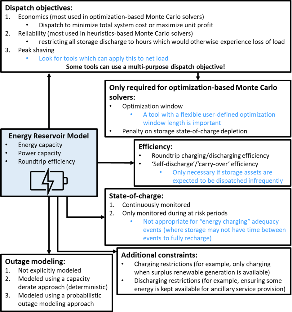
Most tools surveyed use some form of the energy reservoir model (ERM) to model energy storage. This means that each unit can be modeled with a specified energy capacity, power capacity, and roundtrip efficiency. Each unit can charge by consuming energy from the grid, at a rate less than or equal to its power capacity. This consumption is recorded as the stored energy within the unit and can continue until the energy capacity is reached. The unit is also able to provide energy to the grid at a rate constrained by its power capacity, until the stored energy is depleted. The ERM is discussed further in the Technology and System Component Model Selection Guidelines section of this website.
The figure below illustrates the options available for ERM representations across the surveyed tools, with text in blue containing advice on when a certain functionality is important to incorporate. Boxes with numbers indicate where there are several options to choose from, other boxes show constraints to consider. Additional information on storage modeling options is provided below. Note that not every modeling option is necessary for every resource adequacy analysis. The Technology and System Component Model Selection Guidelines section of this website can help guide this choice.
Another method used by tools to represent energy storage involves combining other unit types via the use of custom constraints. One method involves linking a generator and load source together and operating their behavior simultaneously. For example, one tool uses a pair of virtual nodes connected to the grid via one-way lines. One node act as a virtual load with zero VOLL, while the other acts as a virtual generation unit with zero cost. Flow on the two lines is bound by daily or weekly constraints, as well as with weightings to account for losses.
Alternatively, one of the tools surveyed represents storage similarly to thermal plant models. By not accounting for energy capacity, this modeling method essentially assumes that storage duration and initial state-of-charge is adequate to respond for the full duration of an adequacy event. Although this assumption may be suitable under certain conditions, it is likely to fall short in future systems where potential events are longer duration or are close enough together that storage units won't have time to fully recharge in between events. Case studies carried out during the overall initiative pointed to energy storage limits as a driving factor of risk in future years.1,2
These storage models are used by the tools to represent all forms of short duration energy storage. Many tools do not develop separate models for long duration energy storage, with the exception of pumped hydroelectric storage, which is discussed further in the hydropower section of this site.
Read more:
1 EPRI, "Resource Adequacy for a Decarbonized Future, Case Study: Texas (3002027838)," 2023.
2 EPRI, "Resource Adequacy for a Decarbonized Future, Case Study: Western US (3002027834)," 2023.
The vast majority of the tools included in the survey are capable of modelling roundtrip storage efficiency. Storage efficiency is modeled in most tools by applying a flat percentage reduction to the quantity of power consumed and discharged.
Some tools specify a difference between charging/discharging efficiency and ‘carry-over’ or ‘self-discharge’ efficiency. This explicitly accounts for the loss of energy which can occur while in storage. This functionality is particularly useful for systems in which storage which is dispatched infrequently and thus remains charged for extended periods of time, as well as for modeling storage assets that experience substantial amounts of self-discharge, such as thermal storage.
As most tools are using the ERM model, they continuously monitor the energy being utilized in the storage asset, referred to as state of charge (SOC). Once the remaining stored energy is depleted (or in some cases reaches a certain threshold), the unit will be considered empty, and be unavailable to provide power to the system until recharged. However, some tools do not continuously monitor SOC. For example, one tool only investigates storage behavior during time periods that experience loss of load. This tool uses the assumption that all storage will be full prior to the event, with storage only dispatched for reliability purposes. SOC is only monitored for the duration of the event. This approach reduces simulation times. However, it could fail to capture so called “energy charge constrained” adequacy events, defined as events where storage can't appropriately respond to an event because it did not have time in between events to fully recharge.1
Read more:
1 EPRI, "Resource Adequacy for a Decarbonized Future, Case Study: Texas (3002027838)," 2023.
Although almost all real-world storage installations will experience outages, not all resource adequacy tools possess the capability to represent this attribute for storage resources. Length, extent, and duration of storage outages often differs from that of other resources.1 It was noted in conversations with tool providers that this lack of functionality is partly due to a lack of energy storage outage data for practitioners to use. As such, this implementation has not ranked very high on some tool providers’ priority list, even though it may be relatively straightforward to implement if data were available.
Read more:
Energy Storage Dispatch Objectives
Storage discharging, or dispatch, is governed by dispatch objectives, in line with the tool’s overall dispatch algorithm. The three main categories of dispatch objectives are economics, reliability, and peak shaving. Peak shaving refers to restricting dispatch of storage to times of peak demand. Depending on the tool this will either be pure consumer demand (gross demand) or will be the remaining demand to be fulfilled by the grid after variable renewable generation is subtracted (net demand). Economic optimization objectives include dispatching to minimize total system cost or dispatching to maximize unit profit (arbitrage). Reliability dispatching is a heuristics-based approach that typically refers to restricting all storage discharge to hours that would otherwise experience loss of load, and charging the storage unit as soon as the reliability event is over. In some tools, reliability objectives can be constrained further to minimize specific resource adequacy metrics, such as LOLH, LOLEv, or EUE. A number of tools use economic optimization objectives to determine their generation dispatch yet want to ensure storage is also dispatched during reliability events. These tools incorporate a high value of lost load (VoLL) into their models, which ensures that units are dispatched economically, while still minimizing reliability events.
Many storage installations are dispatched for multiple purposes in actual operations.1 In order to represent this, some tools use heuristics such as allocating a certain proportion of capacity to each dispatch purpose. For example, one tool will allow some portion to be modeled as peak shaving, with the rest reserved in case of loss of load. If this functionality is not available for a certain tool, a resource could be modelled as two separate sub-units to mimic a similar effect. Alternatively, some tools allow for multi-purpose dispatch objectives, which often allow for a better representation of actual system behaviors. For example, two tools surveyed use two passes of dispatch optimization, with the first pass minimizing total system cost, and the second pass adjusting the storage dispatch schedule to minimize reliability events. This is often in line with operational practice, in which energy storage dispatch schedule would be adjusted in the case of a system emergency. Although two tools implement this feature, there are slight nuances in the implementation from one to the other. One tool only allows for storage to be re-dispatched in the second pass if it contains enough available energy at the time of the reliability event, while another tool adjusts the pre-event charging schedule to ensure reliability events were mitigated. Although operators often have some level of foresight into times of system stress, the second approach could at times over-optimize storage response.
For tools dispatched using optimization objectives rather than heuristics, the length of the period over which storage operation is optimized, known as optimization window, can dramatically affect the behavior of storage resources, and the resulting RA metrics.1 Resource adequacy studies that consider multiple different types of storage resources may wish to compare the effects of different optimization window lengths. Therefore, the flexibility provided by a tool in choosing optimization window is of particular importance to practitioners.
Finally, some tools have the capability to apply additional constraints to storage charging. Possible constraints include restricting charging to periods with surplus renewable generation, or periods with sufficiently low system marginal cost, as well as ensuring that charging is only scheduled for periods with sufficient surplus generation (after reserves requirements are met). One tool surveyed even allows for the priority order of charging individual units to be modeled.
Read more:
Hybrid Resource Modeling
Hybrid resources provide both generation and storage capacity to the grid. Largely consisting of renewable generation sources paired with co-located storage, these resources allow for variable generation to be stored and used at a later point in time where it will be more valuable to the grid and allow excess generation to be captured for later use rather than spilled.
Hybrid systems can be either AC-coupled or DC-coupled, with DC-coupled configurations allowing for clipped energy to be used to charge the storage unit.1 In order to model DC-coupled systems, tools must be able to account for multiple different inverter efficiencies, as well as differentiate power flow paths.
Various combinations of generation sources and storage types occur in power systems, and the tools surveyed use a variety of different methods to model hybrid resources. Only a few tools use explicit hybrid models, whereas most tools employ constraints between storage and generation models to link their behavior. Characteristics specific to hybrid resources include coupling type, interconnection limits, and grid charging capabilities.
Of the tools evaluated that use explicit hybrid models, one tool’s model consists of a storage capacity that can be ‘charged’ via two inflows: a time-varying exogenous inflow and a grid withdrawal capacity. This time-varying inflow can either be directly input into the grid or can be stored for later use. One efficiency is applied to the entire resource, as it is modeled as a single unit. Another tool with an explicit model possesses less expansive capabilities. While the storage generator that comprises the hybrid plant can be charged from the associated non-dispatchable energy source, it cannot charge from the grid. In this model, the user can specify the capacity of each of the components of the hybrid plant as well as its interconnection limit, allowing for the representation of clipped energy.
Read more:
Hydropower
LEVEL I
Hydropower resources can be represented either through a pre-established generation schedule, or as energy-limited resources scheduled using heuristics. Open-loop PSH systems and cascading hydropower impacts are not represented.
LEVEL II
Hydropower resources can be represented either through a pre-established generation schedule, or as energy-limited resources scheduled using heuristics or optimized using energy allotments or energy trajectories.
Dispatch optimization horizons are user-defined, and energy limitations can be represented as either hard or soft constraints, depending on user choice.
Open-loop PSH systems and cascading hydropower impacts are not represented.
LEVEL III
Hydropower resources can be represented either through a pre-established generation schedule, or as energy-limited resources scheduled using heuristics or optimized using energy allotments, energy trajectories, or water values.
Dispatch optimization horizons are user-defined, and energy limitations can be represented as either hard or soft constraints, depending on user choice.
Open-loop PSH systems can be represented, and important cascading hydropower impacts can be modeled.
All tools included in the survey can represent the three major types of hydroelectric generation: run-of-river (RoR), reservoir, and pumped storage hydropower (PSH), however implementation methods vary widely. Tool capabilities to model these hydropower resources are addressed below, including information on modeling cascading hydropower.
Run-of-River Hydropower
Run-of-river generation is often modeled as a fixed, pre-scheduled output through timeseries. These schedules can be modeled either as constant, or as time varying outputs based on historical generation data, much like wind and solar PV. One of the surveyed tools instead uses the unique approach of representing generation as a probability distribution, derived from historical data. This tool does not use a chronological modeling approach, instead using convolution to assess adequacy. However, across most other tools, run-of-river hydropower generation is either represented as a must-run zero-cost resource, or added to minimum generation constraints for aggregated reservoir hydropower units within the same zone.
Reservoir Hydropower
Most tools represent reservoir hydropower as a form of energy limited dispatchable generation. These units can be dispatched as needed to meet system demand, however, face additional constraints when compared with other dispatchable resources. Energy constraints are imposed due to the unique characteristics of reservoir resources, such as physical reservoir volume limitations, the uncontrollable nature of inflows, and restrictions due to irrigation, environmental, and recreational needs. Indeed, failure to assign additional constraints beyond capacity constraints to reservoir hydropower units would result in the resources being dispatched until they are empty in each optimization period, due to their zero marginal cost, which is not representative of real-life operations, where the energy would have value. Alternatively, one tool represents reservoir hydropower as a probability distribution, derived from historical data, while another tool models it similarly to a thermal generator (considering only its power constraints, and not its energy constraints), assuming that hydro will be dispatched at its maximum level during reliability events.
Energy constraints governing hydropower dispatch are represented differently from one tool to another, with the main methodologies outlined in the following table. More information on energy constraint models can be found in the Technology and System Component Model Selection Guidelines site.
|
Dispatch constraint |
Description |
Computational intensity |
|
Energy Allotments |
A volume of water is assigned to be dispatched by the unit during a given time period |
Low |
|
Energy Trajectories |
A target reservoir level is provided for the start and end of each time period |
Low |
|
Water-values |
Water stored in the reservoir is assigned a cost of dispatch depending on the time of year |
Medium |
|
Water value curve |
Water stored in the reservoir is assigned a value based on the quantity of water currently in the reservoir |
High |
Tools that utilize heuristics for hydropower dispatching such as to minimize LOLE, or to shave peak load, require constraints such as energy allotments or trajectories, which restrict the amount of generation a resource can provide over a given time period. The usage of allotments or trajectories depends on how each tool represents the reservoir of each unit. Some tools that utilize economic dispatch, such as those dispatching to minimize system costs, use constraints such as energy allotments or trajectories, while others assign a value to the water stored within the reservoir. Known as water value, or the shadow value of hydropower, this represents the opportunity cost of dispatching hydropower at a given time rather than waiting until later. Some tools utilize this so that the ‘cost’ of hydropower generation can be compared with other forms of generation.
To determine reservoir hydropower dispatch energy limits annual flow volumes for a given unit are divided among shorter periods such as months or weeks. The expected water inflow for each period is determined using historical data, the weather conditions of a given simulation, or through user input. This inflow volume provides a ‘budget’ for the total reservoir volume available for power generation during a period, subject to environmental, operational or policy constraints that affect maximum and minimum reservoir level. Hydropower energy trajectories are like energy allotment constraints and are often implemented for systems which record reservoir levels rather than flow volumes.
Tools obtain water curves in three main ways: through user input, via the results of initial deterministic runs, or by dynamically assessing the current reservoir status and hydro forecast. While user input and preprocessed curves will require dramatically less computing power, dynamically generated curves can respond much better to system events, and more closely represent real world hydropower operations.
Possible horizons for dispatched hydropower optimization vary across tools, with the most common options being weekly and monthly. Although shorter time frames can reduce computational intensity, hydro data is typically available at monthly resolution. Interpolating this data to weekly resolution can mask inter-week variability in water supply. Shorter optimization horizons could also be less likely to anticipate future needs, such as upcoming droughts, or periods of high demand. As with energy storage modeling, tools that allow for user-defined optimization horizon lengths are preferable to those without this flexibility.
Energy limits can be employed as either hard or soft constraints, with several tools allowing for some carryover of unused capacity to the next month, rather than enforcing complete utilization. The amount of maximum carryover permitted is constrained by the amount of storage space remaining in the reservoir, and environmental or regulatory constraints. A few tools also have the capability to provide updated water use budgets closer to dispatch, and accordingly alter resource allocations. These features allow for better reflection of real-life reservoir operation, however, will also increase computational intensity.
A handful of tools run an in-depth deterministic analysis to set preliminary hydropower profiles, and then allow the hydropower units to deviate from that profile by a certain amount in each of the probabilistic replications to account for short-term uncertainty. In the initial deterministic analysis, forced generator outages are either unaccounted for, or modeled using a simplified fixed derate across all hours of the year, and hydropower dispatch is optimized alongside other system resources. This in-depth optimization is possible for a deterministic run, but would be computationally intensive if done probabilistically.
One of the tools evaluated allows the user to specify an “emergency hydropower” unit class. This type of unit is linked to a reservoir hydropower unit and is assigned both a capacity and energy value upon which the dispatch can draw upon in emergency situations, as well as a payback period during which the dispatched energy must be restored following the emergency event.
Pumped Storage Hydropower
Many of the surveyed tools use a single storage model to represent all types of storage, however some tools either have specific PSH models, or allow for extra constraints to be enacted to represent the characteristics of pumped storage hydropower. This can include the ability to specify distinct operating constraints and costs for every pumping and generating unit within a PSH plant. A couple of the tools surveyed also can incorporate reservoir constraints such as minimum storage level that are variable through time.
Tools using a specific PSH model can model inflows into the upper or lower reservoir, thus realistically representing open-loop PSH units that use rivers as their source of water. This ability is important for the representation of electrical systems with large cascading hydropower systems, in which the outflows of one hydropower unit feed into another unit.
Cascading Hydropower
A key modeling complexity of systems relying on hydropower is the fact that water flows can connect almost any combination of the three main plant types (run-of-river, reservoir, and pumped storage hydropower). When hydroelectric plants are connected, waterflows through one plant affects operations for all connected downstream plants. These connected hydroelectric plant configurations are known as cascading hydropower. Almost half of the tools surveyed as part of this initiative can evaluate a hydroelectric unit as part of a cascading hydropower system. However, modeling cascading hydro operations is highly data and computationally intensive, and as such should be done only where cascading hydropower plays a key role in resource adequacy.
Demand Response
LEVEL I
Demand response is not directly represented as a separate unit type but is incorporated in load timeseries.
LEVEL II
Demand response can be directly represented in the tool as a flexible resource.
A limited number of operating constraints are available.
LEVEL III
Demand response can be directly represented in the tool as either a flexible or shiftable resource. A wide range of operating constraints are available, allowing the user to accurately represent customer fatigue, demand response uncertainty, and the time-varying nature of demand response availability.
Demand response can be incorporated in various ways into a resource adequacy study.1 While some implementations may require specific tool functionality, others do not. For example, many studies incorporate demand response impacts as part of the regional load curve, which is created in pre-processing.
Most of the tools evaluated as part of this initiative can be categorized as Level II, with some within this category allowing for a wider range of operating constraints than others. While a sophisticated modeling capability of demand response is likely not needed in most short-term and medium-term resource adequacy studies, it is becoming increasingly important in long-term adequacy studies, as demand response programs become more widespread and substantial. Further information on demand response modeling options can be found in the Technology and System Component Model Selection Guidelines site.
Read More:
- Modeling New and Existing Technologies and System Components in Resource Adequacy: EPRI Resource Adequacy Assessment Framework. EPRI, Palo Alto, CA: 2023. 3002027830.
- Demand-Side Resources in Resource Adequacy: 2021 – 2023 Research Compilation. EPRI, Palo Alto, CA: 2023. 3002027245.
- Demand Flexibility for Grid Reliability and Resilience: Planning Tool Integration of Demand Flexibility – Phase II. EPRI, Palo Alto, CA: 2023. 3002028252.
Models Available
Demand response can be either flexible, where load decreases or increases its consumption in response to price or dispatch signals without a need for deviations from baseline consumption at a later time, or shiftable, where load can be reduced or increased during a scarcity or high-priced event but any deviations from baseline need to be made up at an earlier or later time.
While flexible demand response representations are commonly found in RA models, shiftable representations are rare. When explicitly modeled, flexible demand response units can be represented using a negative load or pseudo-generator model. Demand response can be either dispatched at a certain activation price (marginal cost) or dispatched heuristically when the system is at risk of a scarcity event. In shiftable models demand response units can be modeled using a pseudo-storage model, requiring the use of additional constraints, including those specifying how quickly energy payback is needed.
Operating Constraints
All explicit demand response modeling approaches rely on several operating constraints to represent unit limitations, the main categories of which are detailed below. Note that some tools have quite a range of operating constraints available while others have none. The constraints can either be directly represented as options available or must be written up by the modeler as custom constraints. As such, there is a great amount of flexibility and nuance as to how they are incorporated from one tool to another. The table below illustrates the main demand response constraints available across the resource adequacy tools surveyed.
The tools evaluated have varying levels of flexibility in terms of the temporal specifications for representing demand response constraints. Some tools allow for all constraints on their system to be specified at any user-defined timestep, while others were more limited. It should be noted that forecasting customer response to demand response programs is nuanced and system- and situation- dependent. As an active area of research, it is anticipated that additional modeling constraints may be needed in future resource adequacy analyses.

In its simplest form, a power constraint consists of a maximum demand response capacity available. In more advanced implementations, this constraint can be customized to account for the time-varying nature of demand response dispatch availability. This customization can either be implemented through an hourly timeseries input by the user, or can be specified by month, by day (for example, only available on weekdays) and/or by hour of day.
This type of constraint is less often employed for demand response programs, but one tool does provide the user with the ability to specify the maximum amount of energy provided by a demand response program, by month or by day. Additionally, the user can specify whether the program allows for excess unused energy to be carried over from one month to another.
Customer fatigue, or the idea that demand response programs may become less effective if they are called on too frequently or for too long, is represented in several different ways depending on the tool employed. Most tools which have this functionality represent it either as a limit on the duration of demand response calls, or a limit on the number of times for which demand response can be called upon. The limit of the duration of demand response calls is sometimes represented as a maximum duration of an individual demand response call or is represented as a limit on the total number of dispatch hours (per day, week, month, or year) or dispatch days (per week, month, or year). Additionally, one tool surveyed allows for the user to set a limit on the number of consecutive days for which a demand response resource can be called upon.
It is worth noting that in many cases, demand response will not drop off sharply after a certain usage threshold is hit, but rather will taper off gradually. One tool surveyed captures this behavior by allowing the user to specify a derate for demand response efficacy after a certain threshold is hit. Even when a tool lacks this explicit operating limitation option, it may be possible to implement it using a workaround. For example, the user could implement different demand response programs switching off a various usage levels, to simulate a partial derate.
At least one tool has the capability of representing uncertainty in price-sensitive load response. In addition to specifying the price at which demand starts to react to market prices, the user can specify an envelope of possible technology response, with the likelihood of responsiveness varying within this envelope.
Demand response is not a uniformly available resource, but rather is dependent on a number of factors. One such factor it may depend on is weather conditions. For example, extreme temperature conditions may reduce the desire of customers to respond to demand response incentives or time-of-use pricing, as maintaining a comfortable indoor environment becomes a principal concern. Additionally, if HVAC systems are not sized appropriately for extreme temperature conditions, they may be run in continuous operation mode at maximum capacity, with no room for duty-cycling, diminishing the ability of programmable and smart thermostats to provide load reduction services.
None of the tools surveyed allow for the capability to tie demand response to temperature profiles, although one tool did allow for it to be tied to load levels.
Key Tool Gaps
Despite rapidly evolving RA tool capabilities, there are still certain gaps that need to be addressed to match evolving RA needs. A set of gaps is listed below, which have been primarily identified through discussions with EPRI project members as well as through individual user experiences across a number of existing RA tools. Further information on RA gaps can be found in the Innovation Gaps page of this site, as well as in the Resource Adequacy Gap Assessment: EPRI Resource Adequacy Assessment Framework document.
Probabilistic RA runs are computationally expensive, especially as resource models are getting more complex and there is an increasing push to consider energy and even flexibility adequacy within probabilistic resource adequacy frameworks.
To this end, many tools have implemented methods to facilitate computational tractability. These include options for parallelization or multi-threading, various methodologies to screen for at-risk adequacy hours, methods to easily simplify or tune the model for probabilistic analysis, and the use of high-performance or cloud-computing. For example, as the dispatch-based Monte Carlo method is very computationally intensive, some users often choose to forgo some of the detailed options it provides to speed up run time and ensure computational tractability. This can be done by manually omitting certain system or unit characteristics (start time, ramp rate, up and down times, etc.) from consideration in the dispatch. Alternatively, several tools in this category can switch between several modeling options to simplify the dispatch when needed (for example, some have an option to switch between a “must run” and “economic constraints” mode).
As resource adequacy moves beyond capacity adequacy into the consideration of energy and flexibility adequacy, the demand for tools having the capability for realistic unit commitment and economic dispatch capabilities is likely grow. This comes at a high computational cost, and even if these features are in theory available in many tools, it may not be computationally feasible to include them for large system studies over multiple years.
Additionally, longer historical records of load and weather data are being considered in resource adequacy analyses than ever before, due to the increased penetration of variable renewable energy resources in many systems, and due to the outsized impact of extreme weather events on system adequacy. Some of these are being adjusted for present and future climate conditions, adding even more uncertainty and potential scenarios. As such, there is a need for resource adequacy tools to be able to handle larger amounts of meteorological data than ever before, and to manage the correlations between weather driven resources efficiently and intuitively.
Although not a tool gap per se, the lack of data availability is in many instances driving a lack of tool development in certain areas. Indeed, if a user does not have the data necessary to implement a certain feature, they will not request this functionality from their tool provider. This chicken-and-egg problem is slowing down tool development in certain areas. Having tool providers continue to be an integral part of resource adequacy research will enable them to play a key role in new methodological developments, rather than being reactive to change.
There are a number of functionalities which are in theory implementable in a given tool, but which would require either the utilization of workarounds or pre- or post-processing on the part of the user. A good example of this is the ability to represent temperature-dependent outage rates: a number of tools allow for this functionality, but separate hourly outage rate profiles for each weather year need to be input, with each weather year run separately, and results then combined in post-processing.
Another example is the calculation of specialized risk metrics, which often requires the user to download large amounts of data and calculate custom metrics using a post-processing script. Many of the tools surveyed as part of this initiative are at level II; if desired, a user can calculate custom-risk metrics or obtain replication-level results, but this requires considerable effort on their part, and may require either the manipulation of large amount of replication-level data in post-processing, or requests for study-specific customizations from the tool provider (a sometimes lengthy and expensive process).
Moreover, resource adequacy tools require a high level of training and expertise to set up, run, and debug. An intuitive user interface, and an up-to-date, clear user manual allow for a better user experience, and ultimately a more robust resource adequacy analysis.
Resource adequacy analysis is only one facet of comprehensive power system planning. A key tool gap identified in discussions with project members is the need to bridge the gap between resource adequacy tools and production cost and capacity expansion tools. Additionally, the ability to integrate gas-electric system modeling in resource adequacy considerations was also identified as a key missing functionality.
A number of the tools evaluated as part of this initiative do allow for use across a number of these planning processes, in particular across resource adequacy analysis, capacity expansion planning, and production cost modeling. This is particularly important as it allows companies to use the same software and the same database across various parts of their long-term planning process, allowing for increased consistency and efficiency.
However, directly combining these analyses, while mathematically possible, would result in major computational tractability issues. As such, tools must ensure a seamless transition from one process to the next and should have automation capabilities in place to allow users to easily use the full suite of capabilities. For example, a useful tool functionality would be the automation of the round-trip analysis required for a capacity expansion buildout which optimizes economic efficiency while also guaranteeing a consistent reliability output.